ATAC-Seq Data Analysis
Introduction
To understand Assay for Transposase-Accessible Chromatin using sequencing (ATAC-Seq), let us take a moment to explore the spatial organization of the genome. The genome (circa 1.8 meters in length) is squished and squeezed inside a 6 micrometer (µm) nucleus. This follows that there is no chance that the DNA would stay linear in terms of layout. It will exhibit folds, twists, turns, and intersections ( What a messy piece of road; I would never want to drive over it! ). Imagine taking a length of loose cotton thread and fitting it in your trouser pocket. You'll know what I mean.
With such a scenario, the interactions between distant genomic sections are bound to happen as they come in close contact. It is neither a predicament nor inadvertent, rather a programmed mechanism that is peculiar to each cell type. That is why a nerve cell functions differently than a muscle cell. The bottom line is that even though the genome is same throughout,the interactome is different for disparate cells, and hence the diversity in function and phenotype. This has been the key driver of the single-cell studies [1].
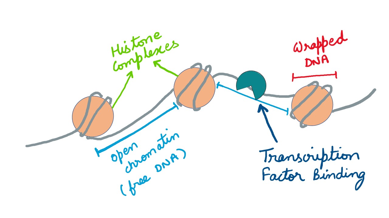
It is clear that the landscape of the genome, seemingly random, is immaculately structured inside the nucleus. Then there are domains, subdomains, compartments, etc. [2], details of which are beyond the scope of this primer. But, let's get back to ATAC-Seq. Intuitively, the compaction of the DNA is on the utmost importance and there are several phases over which this mechanism is laid. At the base-level, the DNA is wrapped around the histone proteins (this fraction of DNA accounts for ~147 bases, called the nucleosome), and is only accessible when set free from the tangle. Broadly, strings of such wraps constitute a chromatin and the role of ATAC-Seq is to study accessibility of chromatin and hence examine regulators of gene expression. A fair description about this technology could be found here . ATAC-Seq is a preferred methodology when compared to the contemporaries as FAIRE-Seq and DNase-Seq , for its efficiency.
The data is from a human cell line of purified CD4+ T cells, called GM12878 [3]. The original dataset had 2 x 200 million reads and would be too big to process in a training session, so we downsampled the original dataset to 200,000 randomly selected reads. We also added about 200,000 reads pairs that will map to chromosome 22 to have a good profile on this chromosome, similar to what you might get with a typical ATAC-Seq sample (2 x 20 million reads in original FASTQ). Furthermore, we want to compare the predicted open chromatin regions to the known binding sites of CTCF . It is used as a positive control for assessing if the ATAC-Seq experiment is good quality. Good ATAC-Seq data would have accessible regions both within and outside of TSS, for example, at some CTCF binding sites. For that reason, we will download binding sites of CTCF identified by ChIP in the same cell line from ENCODE (ENCSR000AKB, dataset ENCFF933NTR).
Assimilating Data and Metadata
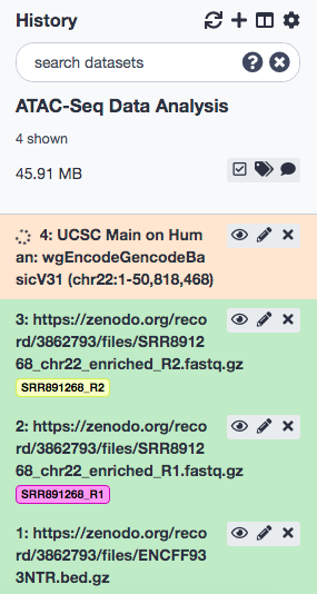
As a norm, we will create a new History (session) for this data analysis module. Further, we load the data from the following web-links.
- https://zenodo.org/record/3862793/files/ENCFF933NTR.bed.gz
- https://zenodo.org/record/3862793/files/SRR891268_chr22_enriched_R1.fastq.gz
- https://zenodo.org/record/3862793/files/SRR891268_chr22_enriched_R2.fastq.gz
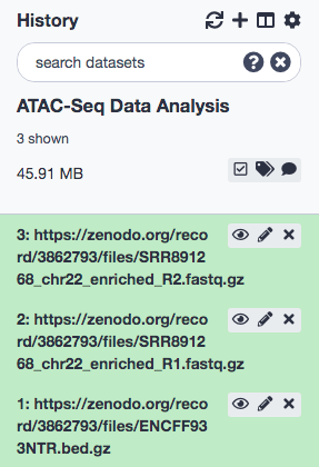
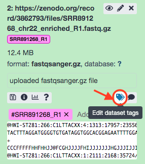
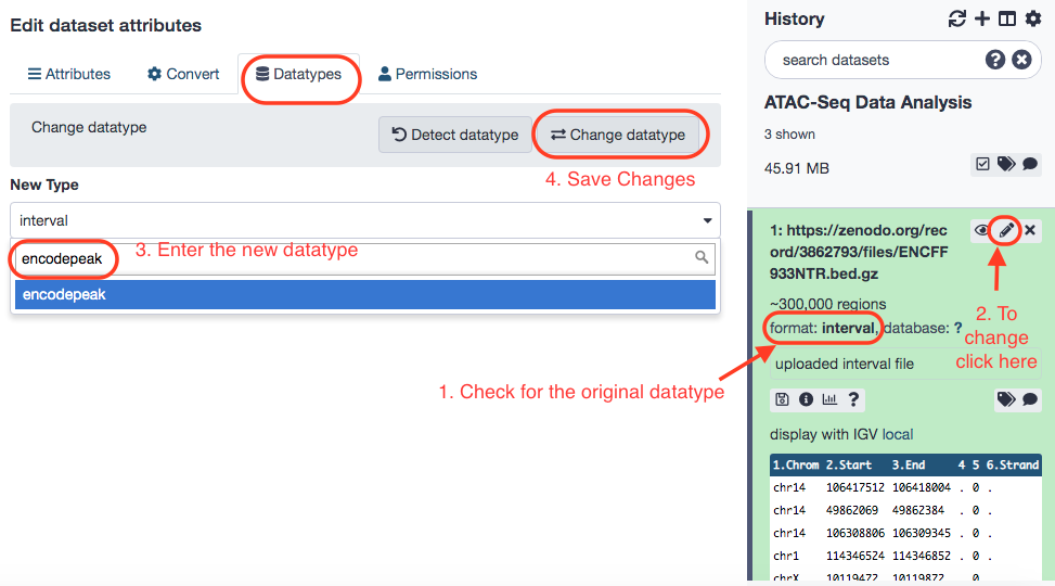
With the data successfully imported into Galaxy, we add a tag called #SRR891268_R1 to the R1 file and a tag called #SRR891268_R2 to the R2 file. (Note: Tags are extremely useful in flagging components that are part of a result from a tool. This could potentially be a life-saver when it comes to lengthy workflows, where it is hard to be track of, say, input data that was imported in the beginning of the pipeline). Also, check that the datatype of the 2 FASTQ files is fastqsanger.gz and the peak file (ENCFF933NTR.bed.gz) is encodepeak. The procedures are illustrated below.
Next, we will obtain gene annotation (hg38) for chromosome 22 genes (names of transcripts and genomic positions) using the UCSC Table Browser . This step could be explicitly carried out and the results are imported to the Main Galaxy . The results can eventually be imported to the local Galaxy.
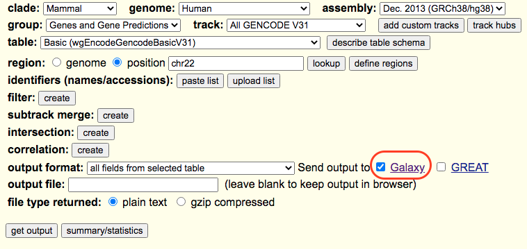

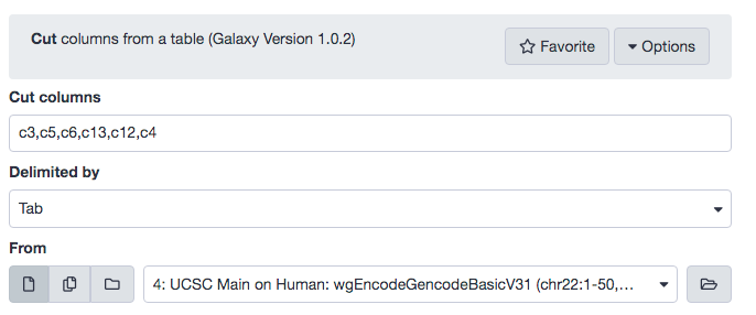
This table contains all the information but is not in a BED format. To transform it into BED format we will cut out the required columns and rearrange. We will use the Cut which is a default tool available in Galaxy. The following parameters must be used.
- “Cut columns”: c3,c5,c6,c13,c12,c4
- “Delimited by”: Tab
- “From”: UCSC Main on Human: wgEncodeGencodeBasicV31 (chr22:1-50,818,468)
Examine the result for accuracy and rename as chr22 genes, and change the datatype to bed. Recall that we are particularly interested in Chromosome 22.
Quality Control
As a foremost standard measure, a quality check ensures that the data is potent to delivery acceptable results. We shall now perform a run of FASTQC , to examine the grade of reads and presence of adapter sequences. Before the run, let us rename the files for convenience. Also, we could choose either of the files or both, by selecting single-file or multiple-files mode, respectively.
Exercise
- Examine the FASTQC results.
Trimming Reads
To trim the adapters we provide the Nextera adapter sequences to Cutadapt tool. The forward and reverse adapters are slightly different. We will also trim low quality bases at the ends of the reads (quality less than 20). We will only keep reads that are at least 20 bases long. We remove short reads (< 20bp) as they are not useful, they will either be thrown out by the mapping or may interfere with our results at the end. The following values to options shall be instantiated.
- “Single-end or Paired-end reads?”: Paired-end
- “FASTQ/A file #1”: SRR891268_chr22_enriched_R1.fastq
- “FASTQ/A file #2”: SRR891268_chr22_enriched_R2.fastq - In “Read 1 Options”:
- “Source”: Enter custom sequence
- “Enter custom 3’ adapter name (Optional if Multiple output is ‘No’)”: Nextera R1
- “Enter custom 3’ adapter sequence”: CTGTCTCTTATACACATCTCCGAGCCCACGAGAC - In “Read 2 Options”: - In “3’ (End) Adapters”: - “Insert 3’ (End) Adapters”
- “Source”: Enter custom sequence
- “Enter custom 3’ adapter name (Optional)”: Nextera R2
- “Enter custom 3’ adapter sequence”: CTGTCTCTTATACACATCTGACGCTGCCGACGA - In “Filter Options”:
- “Minimum length”: 20 - In “Read Modification Options”:
- “Quality cutoff”: 20 - In “Output Options”:
- “Report”: Yes
- In “3’ (End) Adapters”:
- “Insert 3’ (End) Adapters”
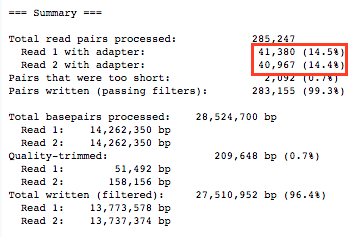
We get approximately 14% reads with adapters.
With the filtered reads, we run FASTQC again and analyze the results. It is to be noticed that the adapter content is completely removed from the reads.
Mapping Reads to Reference Genome
Mapping reads to the reference genome aids to determine the genomic regions where the reads align. We shall now be using Bowtie2 with the following options.
- “Is this single or paired library”: Paired-end
- “FASTQ/A file #1”: select the output of Cutadapt tool “Read 1 Output”
- “FASTQ/A file #2”: select the output of Cutadapt tool “Read 2 Output”
- “Do you want to set paired-end options?”: Yes
- “Set the maximum fragment length for valid paired-end alignments”: 1000
- “Allow mate dovetailing”: Yes
- “Will you select a reference genome from your history or use a built-in index?”: Use a built-in genome index
- “Select reference genome”: Human (Homo sapiens): hg38 Canonical
- “Select analysis mode”: 1: Default setting only
- “Do you want to use presets?”: Very sensitive end-to-end (--very-sensitive)
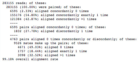
- “Save the bowtie2 mapping statistics to the history”: Yes
(P.S. For justifications of the above choices, please visit the original tutorial; see [5]). Also note that Bowtie2 considers a read as multi-mapped even if the second hit has a much lower quality than the first one. Another reason is that we have reads that map to the mitochondrial genome. The mitochondrial genome has a lot of regions with similar sequence.
Filtering Mapped Reads
The vulnerability of ATAQ-Seq to the mitochondrial genome is high, because the mitochondrial genome is deprived of nucleosomes [4]. So, a wise choice is to remove these reads, alongwith reads with low quality and the ones that are not properly paired. For the same purpose, we use the tool Filter from the repository bamtools_filter, and mark the options as represented in the following screenshot.
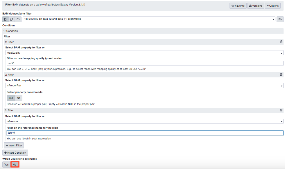
You'll notice the size difference in the input (27.9 MB) and output (15.1 MB) BAM files from the tool. (Note: The tool Samtools idxstats could be used on the output of Bowtie2 tool (BAM file), to tabulate the number of reads that map to a paritcular chromosome).
Filter Duplicate Reads
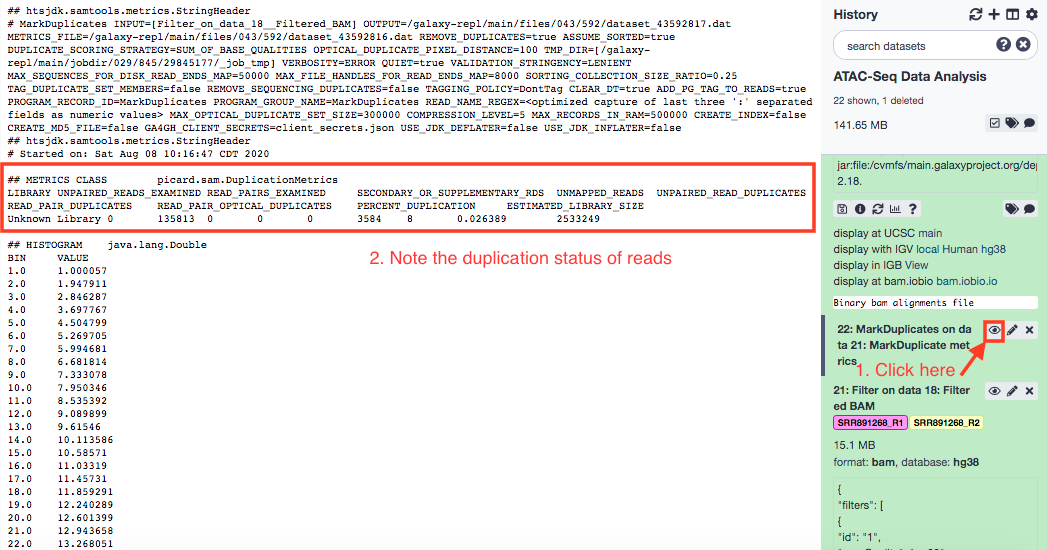
Fundamentally, Polymerase Chain Reaction (PCR) has been designed to replicate DNA segments, and that could engender duplicacy in the pool of reads. This redundancy depicts different reads mapping exactly to the same genomic region. Such PCR duplicates are to be removed using MarkDuplicates tool, from the picard repository.
Use the following parameters.
- “Select SAM/BAM dataset or dataset collection”: Select the output of Filter tool “BAM”
- “If true do not write duplicates to the output file instead of writing them with appropriate flags set”: Yes
The second parameter marked as "Yes" is the one that actually deletes the duplicates. If otherwise, the duplicates are only flagged.
Check Insert Sizes
Next, we are going to check the insert size, i.e. distance between paired-end reads (R1 and R2). This tells us the size of the DNA fragment, the read pairs came from. The fragment length distribution of a sample gives a very good indication of the quality of the ATAC-Seq. We shall be using CollectInsertSizeMetrics from the repository, picard.
Try the following choices for paramaters.
- “Select SAM/BAM dataset or dataset collection”: Select the output of MarkDuplicates tool “BAM output”
- “Load reference genome from”: Local cache
- “Using reference genome”: Human Dec. 2013 (GRCh38/hg38) (hg38)
Figure 1: Fragment Size Distribution Simple put, a transposase is an enzyme that plucks the DNA and moves it to a different place. The above graphic shows, in descending order, the length of DNA fragments from an ATAC-Seq experiment. This implies that distribution of DNA lengths that are nucleosome-free, between two histone-wraps, between three histone-wraps, and so on (from right to left). 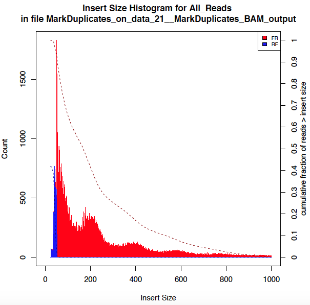
Note: The legends in the aforementioned graphic, FR stands for forward reverse orientation of the read pairs, meaning, your reads are oriented as -> <- so the first read is on the forward and the second on the reverse strand. RF stands for reverse forward oriented, i.e., <- ->.
Peak Calling
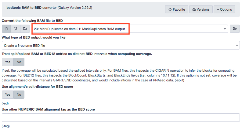
In this module, we commence with the post-processing of the samples. The first stage is peak-calling ; peaks are distinguished piles of reads. It is very important at this point that we center the reads on the 5’ extremity (read start site) as this is where Tn5 (the transposase) cuts. You want your peaks around the nucleosomes and not directly on the nucleosome. For this task, we shall be using MACS2 , from the repository macs2. The first requirement, however, is to convert BAM file to a BED file. Use bedtools BAM to BED converter from the repository bedtools.
Now, we execute MACS2 callpeak with the following options:
- “Are you pooling Treatment Files?”: No
- “Do you have a Control File?”: No
- “Format of Input Files”: Single-end BED
- “Effective genome size”: H. sapiens (2.7e9)
- “Build Model”: Do not build the shifting model (--nomodel)
- “Set extension size”: 100
- “Set shift size”: -50 - “Additional Outputs”:
- Check Peaks as tabular file
- Check Peak summits
- Check Scores in bedGraph files - In “Advanced Options”:
- “Composite broad regions”: No broad regions
- “Use a more sophisticated signal processing approach to find subpeak summits in each enriched peak region”: Yes
- “How many duplicate tags at the exact same location are allowed?”: all
Also, add a tag called #MACS2_cov to the output called MACS2 callpeak …(Bedgraph Treatment).
Visualization of Coverage
Convert to Bigwig
To make the output file valid for downstream use, we first convert it to bigwig format. We use the tool Wig/BedGraph-to-bigWig converter.
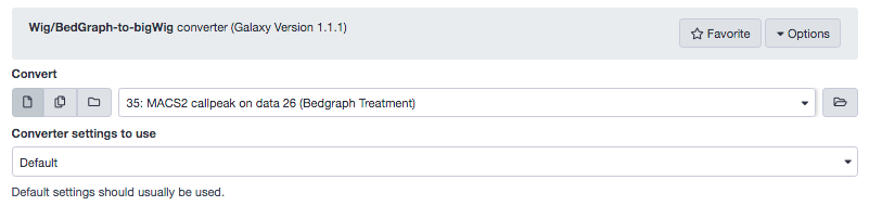
Rename the output file to MACS bigwig.
Sort CTCF Peaks
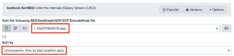
We can use several exploratory tools to visualize specific genomic regions; a genome browser like IGV or UCSC Browser , or choose pyGenomeTracks to make graphics. In the module, we employ pyGenomeTracks. The pyGenomeTracks tool needs all BED files sorted , thus we sort the CTCF (our protein of interest, that binds to the open chromatin) peaks.
Create heatmap of coverage at TSS with deepTools
computeMatrix
The output of this function is a pre-requisite to the plotHeatmap function. It delivers a matrix with features to plot.
Input the following values of parameters in computeMatrix.
-
- In “Select regions”:
- - “Select regions”
- “Regions to plot” : chr22 genes
- “Sample order matters” : No
- “Score file” : MACS2 bigwig
- “computeMatrix has two main output options” : reference-point
- “The reference point for the plotting” : beginning of region (e.g. TSS)
- “Show advanced output settings” : no
- “Show advanced options” : yes
- “Convert missing values to 0?” : yes
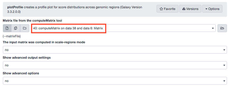
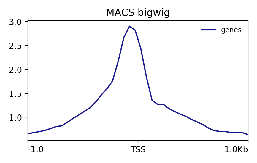
plotProfile
This visualization gives the mean coverage around the TSS.
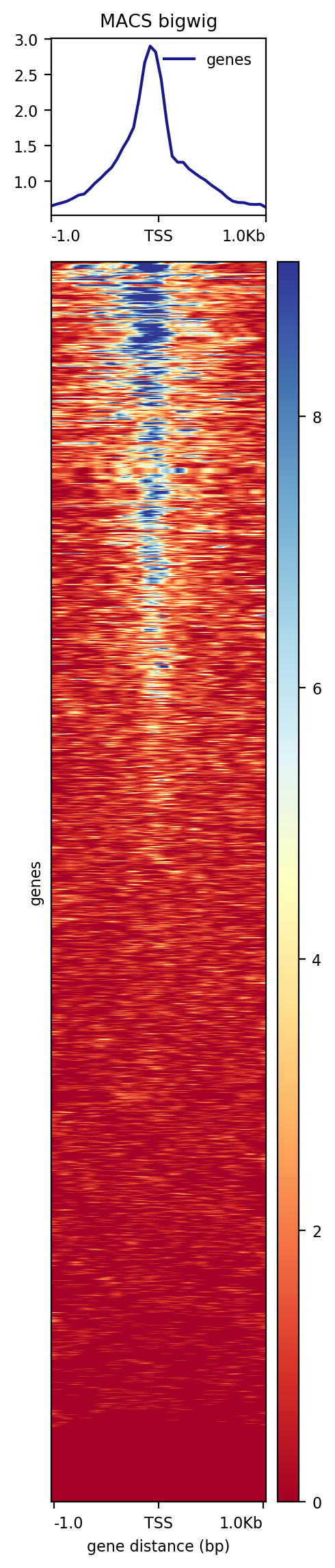
plotHeatmap
This function scales the output of the plotProfile with a heatmap. Each line will be a transcript (instances from chr22 genes). The coverage will be summarized with a color code from red (no coverage) to blue (maximum coverage). All TSS will be aligned in the middle of the figure and only the 2 kb around the TSS will be displayed. Another plot, on top of the heatmap, will show the mean signal at the TSS.
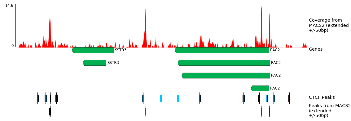
Visualise Regions with pyGenomeTracks
Load the tool and instantiate the following constraints.
- “Region of the genome to limit the operation”: chr22:37,193,000-37,252,000 - In “Include tracks in your plot”:
- “1. Include tracks in your plot”
- “Choose style of the track”: Bigwig track
- “Plot title”: Coverage from MACS2 (extended +/-50bp)
- “Track file bigwig format”: MACS2 bigwig.
- “Color of track”: Select the color of your choice
- “Minimum value”: 0
- “height”: 5
- “Show visualization of data range”: Yes
- “Choose style of the track”: NarrowPeak track
- “Plot title”: Peaks from MACS2 (extended +/-50bp)
- “Track file bed format”: MACS2 callpeak(narrow Peaks)
- “Color of track”: Select the color of your choice
- “display to use”: box: Draw a box
- “Plot labels (name, p-val, q-val)”: No
- “Choose style of the track”: Gene track / Bed track
- “Plot title”: Genes
- “Track file bed format”: chr22 genes
- “Color of track”: Select the color of your choice
- “height”: 5
- “Put all labels inside the plotted region”: Yes
- “Allow to put labels in the right margin”: Yes
- “Choose style of the track”: NarrowPeak track
- “Plot title”: CTCF peaks
- “Track file bed format”: Select the dataset bedtools SortBED of ENCFF933NTR.bed
- “Color of track”: Select the color of your choice
- “display to use”: box: Draw a box
- “Plot labels (name, p-val, q-val)”: No
- “Insert Include tracks in your plot”
- “Insert Include tracks in your plot”
- “Insert Include tracks in your plot”
We realize something like this.
References
- Zheng, H., Xie, W. The role of 3D genome organization in development and cell differentiation. Nat Rev Mol Cell Biol 20, 535–550 (2019). https://doi.org/10.1038/s41580-019-0132-4
- Rowley, M. J., & Corces, V. G. (2018). Organizational principles of 3D genome architecture. Nature reviews. Genetics, 19(12), 789–800. https://doi.org/10.1038/s41576-018-0060-8
- Buenrostro, J. D., P. G. Giresi, L. C. Zaba, H. Y. Chang, and W. J. Greenleaf, 2013 Transposition of native chromatin for fast and sensitive epigenomic profiling of open chromatin, DNA-binding proteins and nucleosome position. Nature Methods 10: 1213–1218. 10.1038/nmeth.2688
- Taanman, J.-W. (1999). The mitochondrial genome: structure, transcription, translation and replication. Biochimica et Biophysica Acta (BBA) - Bioenergetics, 1410(2), 103–123. https://doi.org/https://doi.org/10.1016/S0005-2728(98)00161-3
- Lucille Delisle, Maria Doyle, Florian Heyl, 2020 ATAC-Seq data analysis (Galaxy Training Materials). /training-material/topics/epigenetics/tutorials/atac-seq/tutorial.html Online; accessed Sat Aug 08 2020
- Batut et al., 2018 Community-Driven Data Analysis Training for Biology Cell Systems 10.1016/j.cels.2018.05.012