
Classification in Machine Learning
Introduction
In this tutorial, we shall learn to deal with classification problems using Galaxy. We shall examine Logistic Regression (a linear classifier), the Nearest Neighbor (a nonlinear classifier), Support Vector Machines , Random Forest and other ensemble classifiers, with data visualization for each application. We will also explore ways to minimize the cost function.
Supervised Learning
Classification is a supervised learning method in machine learning and the algorithm which is used for this learning task is called a classifier. The idea is to map data instances to certain pre-defined class labels, and this is carried out by perusing nuances from the attributes of the input data. My best intuition that fits the theme and is often reciprocated on the adverts in the public domain, is that of Garbage Classification ; a simple notion that has a tremendous impact in the recycling of waste products. So depending on the physical and chemical properties of a junk, it is dispensed in the appropriate (color-coded) bin.
To explore this theme, we will perform a case study on cheminformatics data, arguing if a chemical substance is biodegradable; a purposeful examination that aligns to the environmental safety aspects. A database (Mansouri et al.) of compounds is collected for which the property of interest is known. For each compound, molecular descriptors are collected which describe the structure (for example: molecular weight, number of nitrogen atoms, number of carbon-carbon double bonds). Using these descriptors, a model is constructed which is capable of predicting the property of interest for a new, unknown molecule. This database contains 1055 molecules, together with precalculated molecular descriptors.
Data Sourcing
We have the data pre-clustered into training and testing sets and could be downloaded into the Galaxy instance via the following links:
- https://zenodo.org/record/3738729/files/train_rows.csv
- https://zenodo.org/record/3738729/files/test_rows_labels.csv
- https://zenodo.org/record/3738729/files/test_rows.csv
As usual, we rename the datasets for our convenience. Now that we have the data, we will get into the core of our analysis. Let us begin by applying the logistic regression classifier to model the data.
Logistic Regression Classifier
The logistic function aims to calculate the weight(coefficient/ slope) and bias(error/ intercept) for the line that will fit the data in question, and innately, project the predicted class labels over the true class labels. The dissimilarity or the distance between these respective labels is the loss/ cost function. The second thing we need is an optimization algorithm for iteratively updating the weights so as to minimize this loss function. The standard algorithm for this is gradient descent.
We will use the tool Generalized linear models from the repository sklearn_generalized_linear, and make the following choices for paramaters.
- “Select a Classification Task”: Train a model
- “Select a linear method”: Logistic Regression
- “Select input type”: tabular data
- “Training samples dataset”: train_rows
- “Does the dataset contain header”: Yes
- “Choose how to select data by column”: All columns EXCLUDING some by column header name(s)
- “Type header name(s)”: Class
- “Dataset containing class labels”: train_rows
- “Does the dataset contain header”: Yes
- “Choose how to select data by column”: Select columns by column header name(s)
- “Select target column(s)”: Class
We rename the generated file to LogisticRegression_model and proceed towards making predictions by applying the model on test data. That will lead us to determine the accuracy of the model.
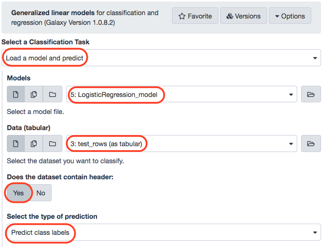
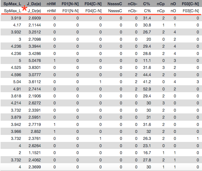
Note: The training data has features as well as the corresponding class-labels. Although, the test data we use for making predictions is without class-labels (just values for features). Additionally, the data we employ for testing model accuracy is just the class-labels for test data.
We rename the results of the logistic regression model to LogisticRegression_result, and remove the header from the test_rows_labels file.

Let us view the results.
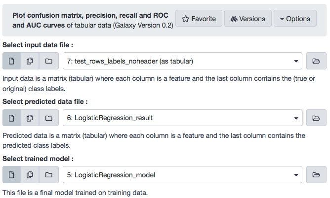
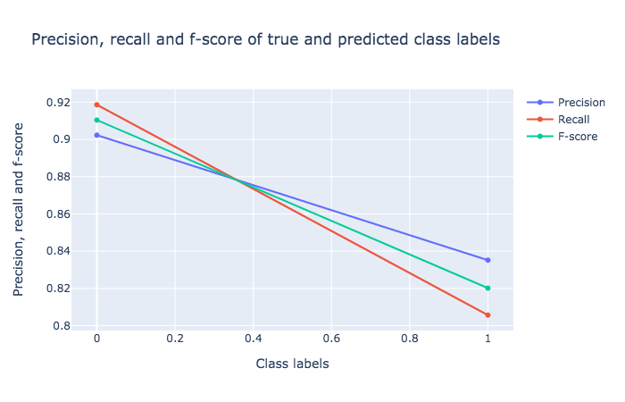
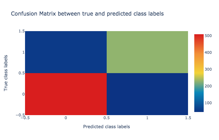
The visualization tool created three plots for, viz. Confusion Matrix, Precision, recall and F1 score , and Receiver Operator Characteristics (ROC) and Area Under ROC (AUC) , as depicted below.

K-Nearest Neighbor (KNN) Classifier
In this classification scheme, a data sample is assigned to the class that is most common to its neighbors, the variable k defines the number of nearest neighbors to look out for. This value is critical and while a small k could induce a lot of noise, a larger k might well contain points from other classes and engender erroneous classification. A prefered way is to run the classifier with varying k and then choose the model with optimum error.
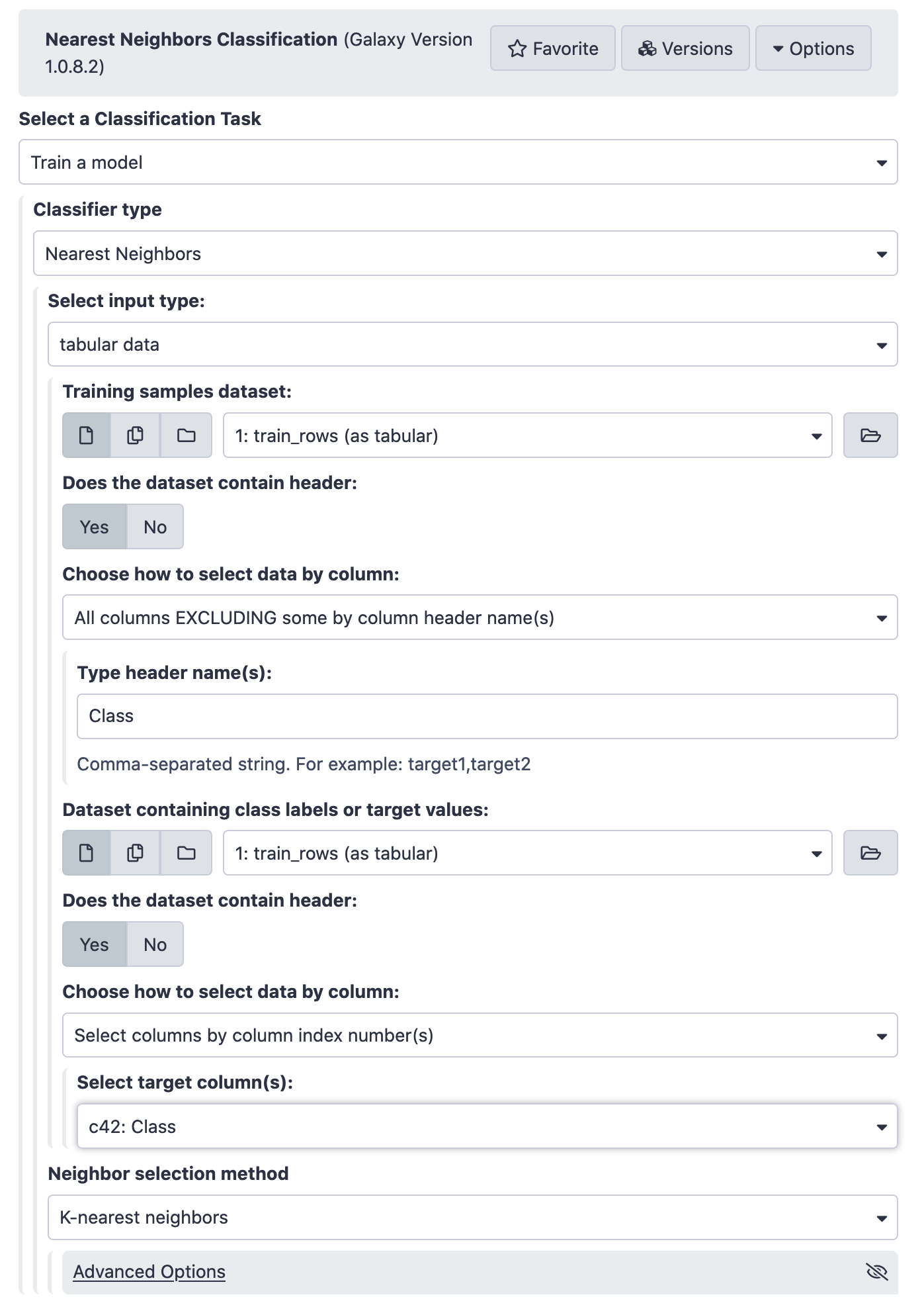
To run this algorithm in Galaxy, we'll install the tool Nearest Neighbors Classification from the repository sklearn_nn_classifier. As you would find out, the classifier was trained with k = 5, which is the default value.
With the model in place now, let us use it for the test data and gauge it's potency.

Visualizing Results
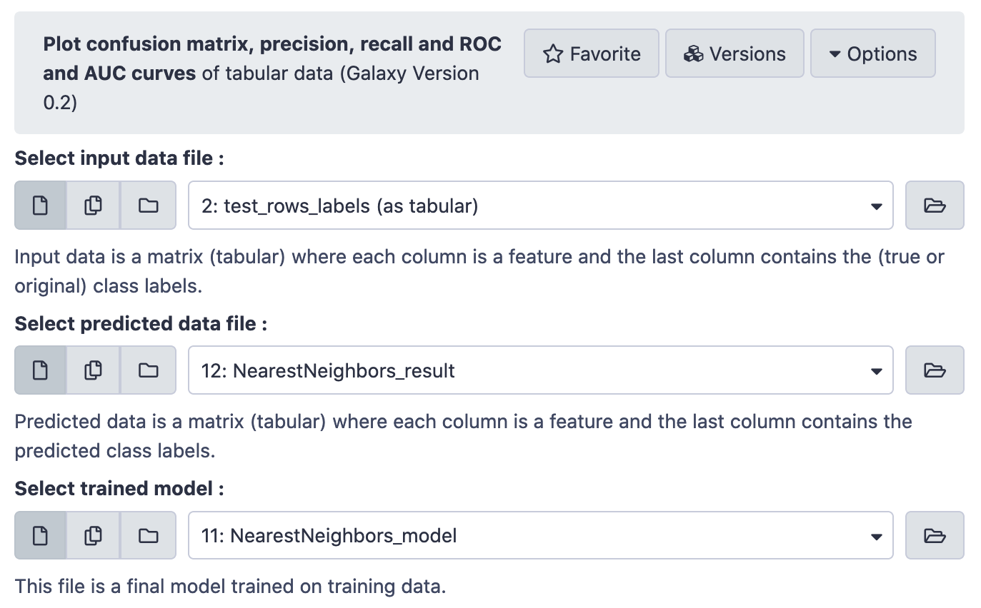
Subsequently.

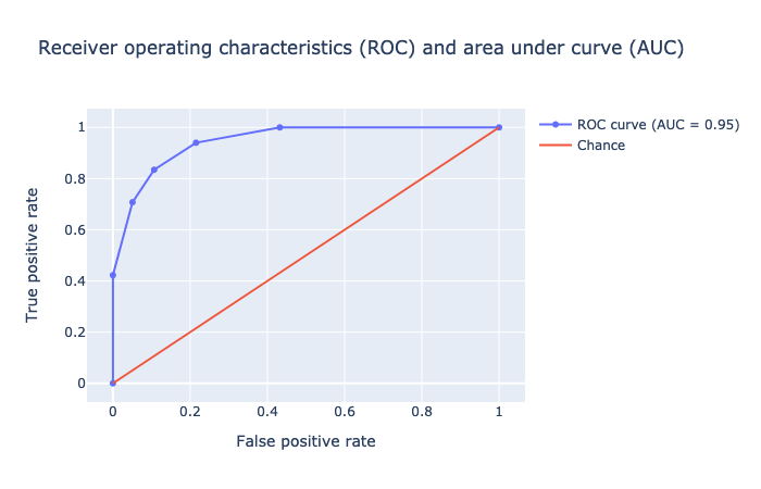
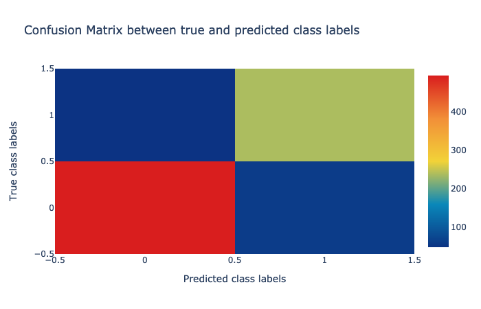
As you would note, the accuracy of this classifier (AUC = 0.95) is tad better than the logistic regression model (AUC = 0.94).
Support Vector Machines (SVMs)
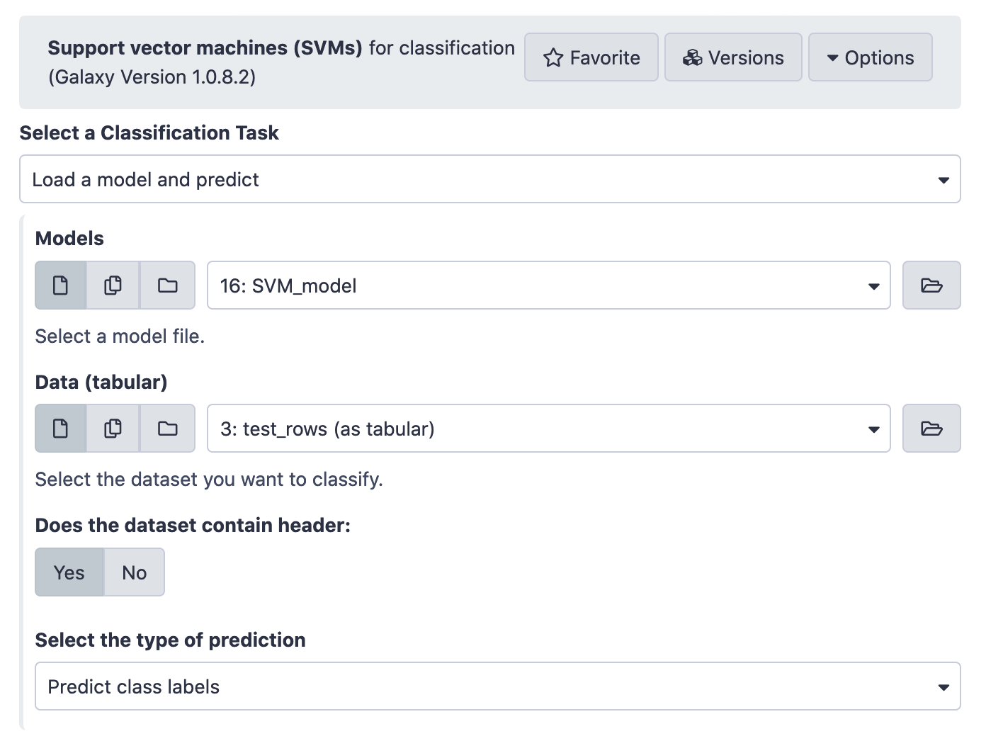
A primer for this classification scheme is available here . Let us dive right into the application.

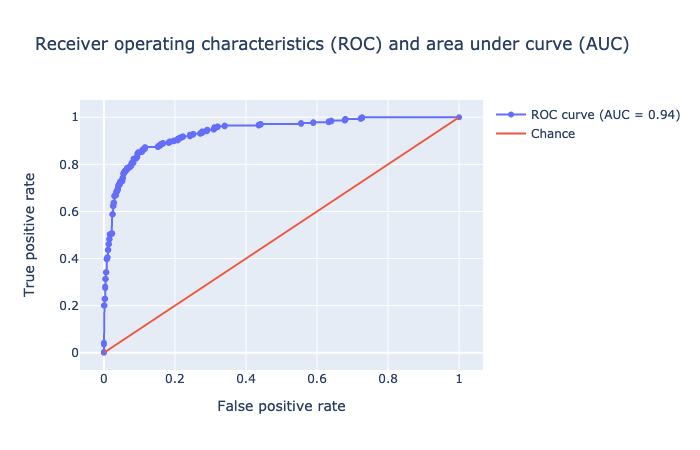
The SVM model learns the coefficients of the hyperplane with the maximal margin in the kernel space, between classes. Let us apply the model on test data and then visualize the results.
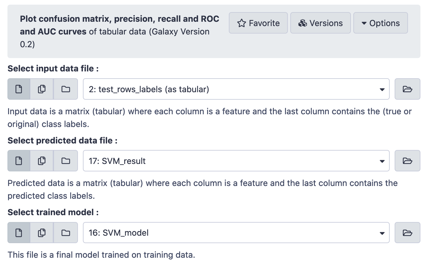
Again,


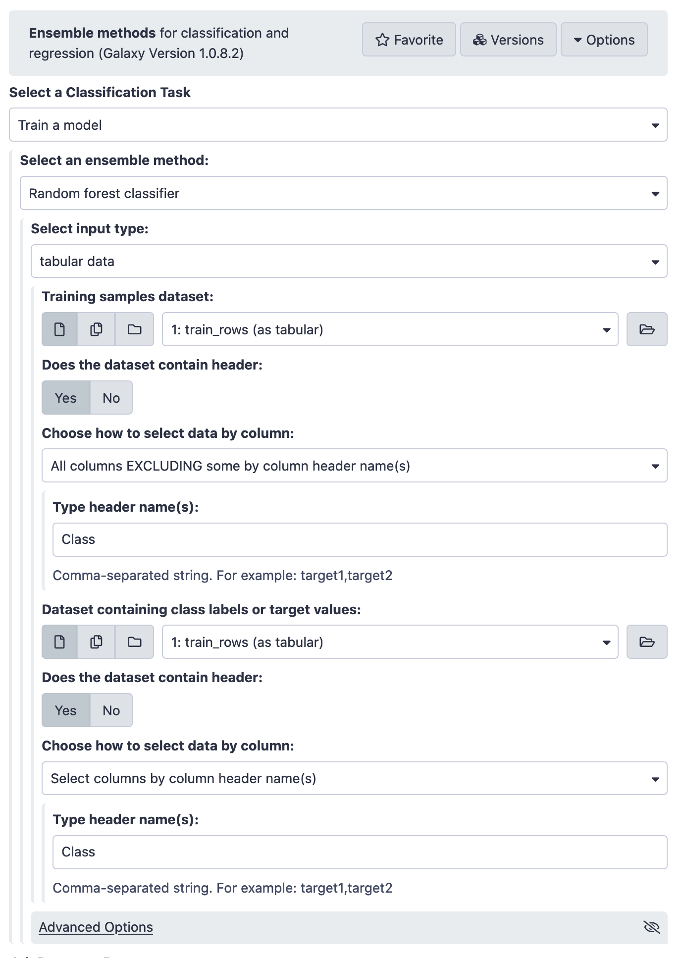
Random Forest
An ensemble of decision trees, this classifier improvises the overall results by aggregating results from a multitude of learning models. It is a "boosting and bagging" methodology that iteratively minimizes error. See this presentation for reference. The problem of overfitting is least likely in an ensemble method as it generalizes well, being trained on several instances of the data.
Building Model
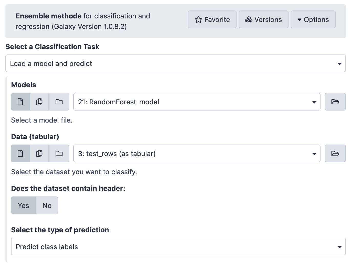
Application on Test Data
Visualizing Results
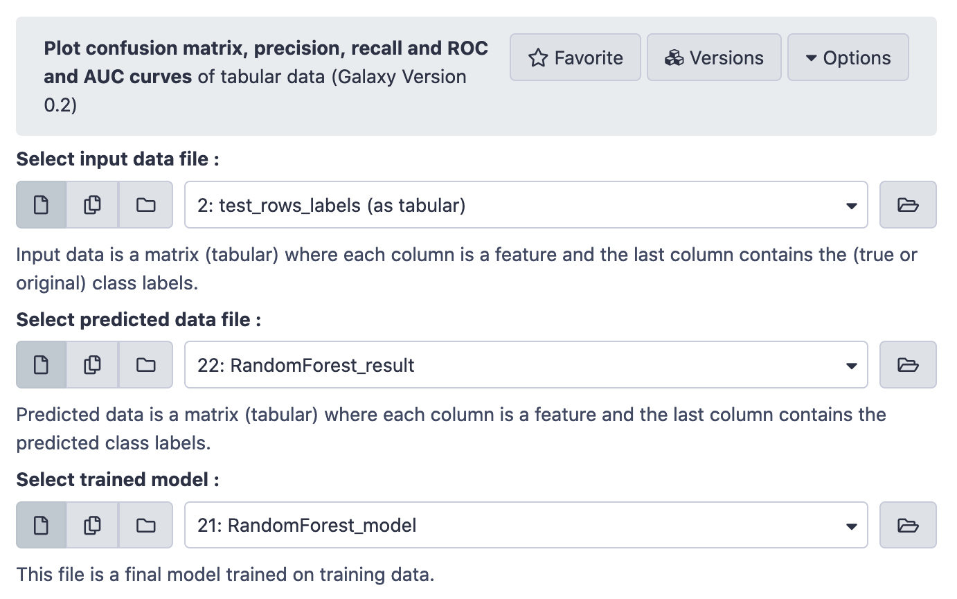
Finally,
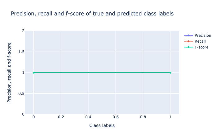
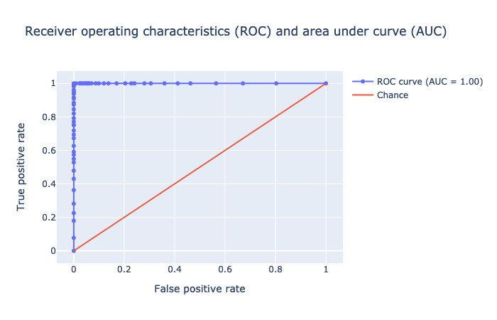

The results are perfect. The AUC = 1.0 indicates absolutely no error.
Creating a Data Processing Pipeline | Ensemble Classifier
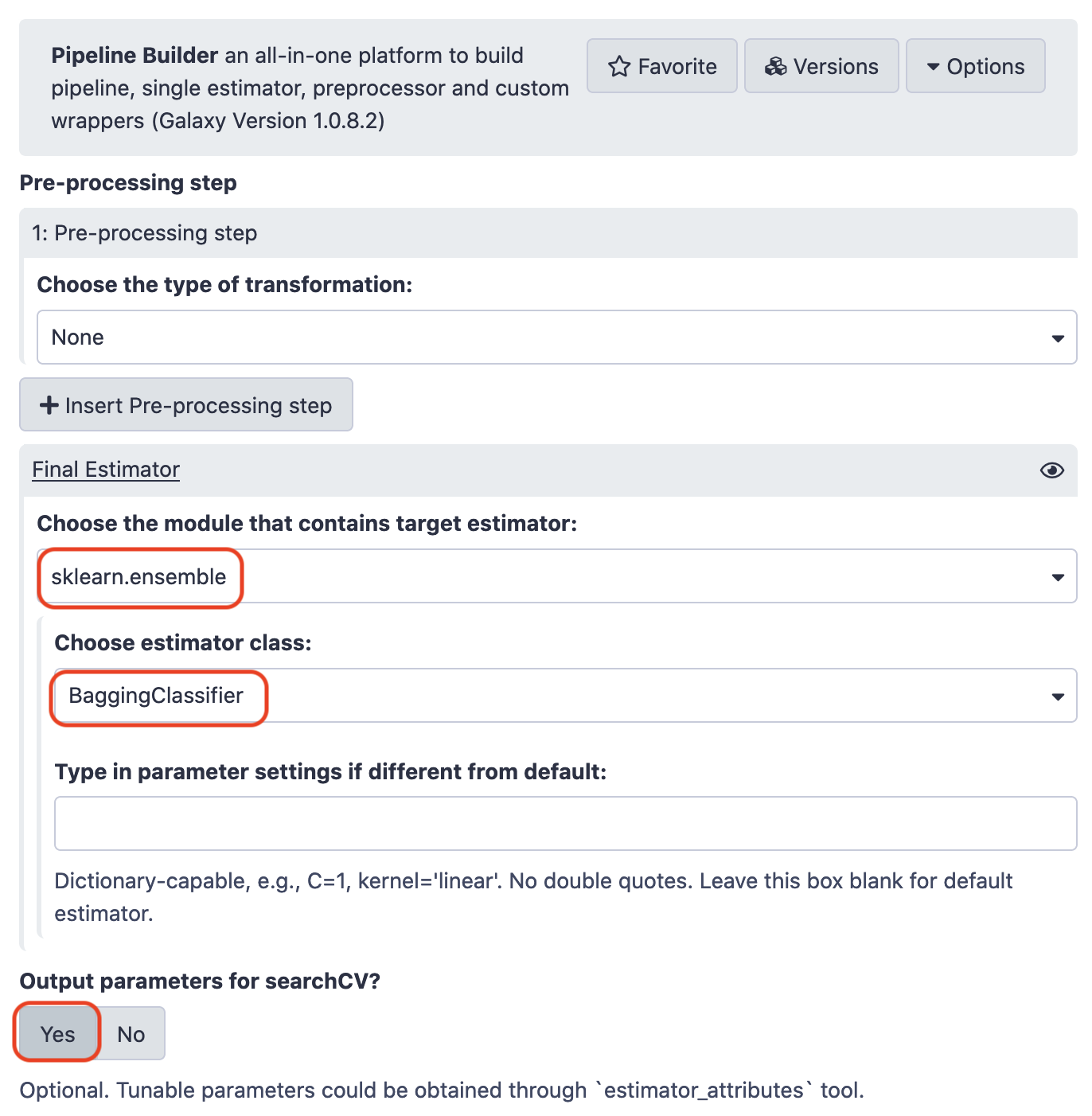
Pipeline Builder
We need a list of hyperparameters of the estimators. This is the output of pipeline builder that shall eventually be fed to the Hyperparameter search tool. However, we shall particularly focus on the constraint, n_estimators, as this defines the number of stages for the "bagging" operation. As we know, "bagging" allows for aggregation of results for a concensus. In addition, it must be examined that this value is neither too high (as we'll be making unnecessary expenditure on processing and time), neither too low (so that the accuracy is hampered). The Hyperparameter search tool gives us just the optimal number we need. (Note: The default value of n_estimators for this regressor is 10)
Hyperparameter Search
Try the following choices.

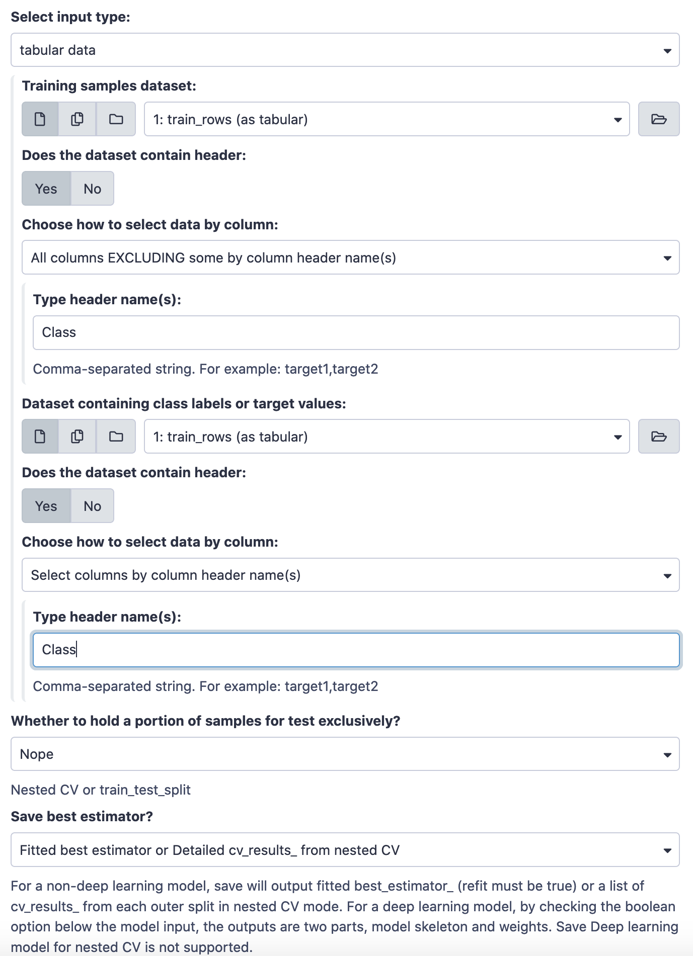
This run results in two files; the model (zip file) and the hyperparameter values (tabular file). Have a look at the tabular file.

The column mean_test_score gives the accuracy for the model, corresponding to the given parameter value. So, although the default value is 10, yet 50 gives us a better model. That is exactly why it is important to tune the model in accord to these parameters to give us the optima. Agin, we'll make the prediction with the new model.
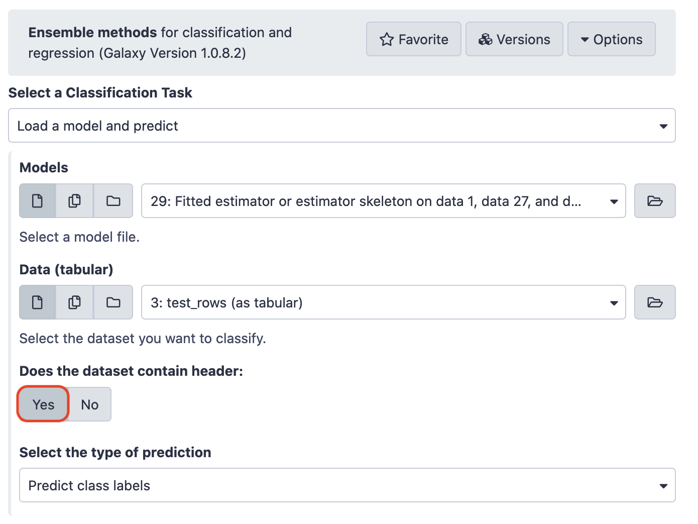
Visualization of Results
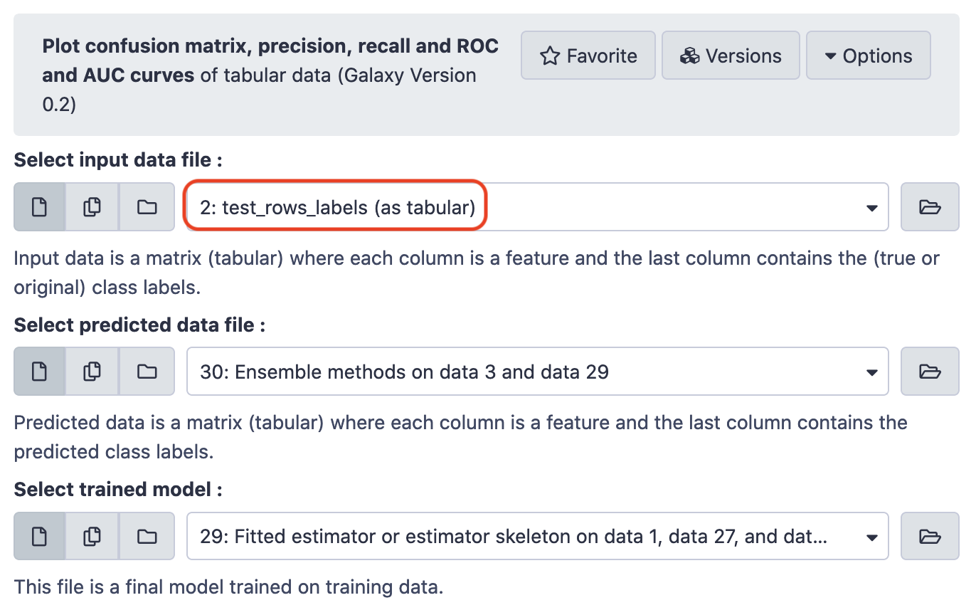
Pulling the plots,


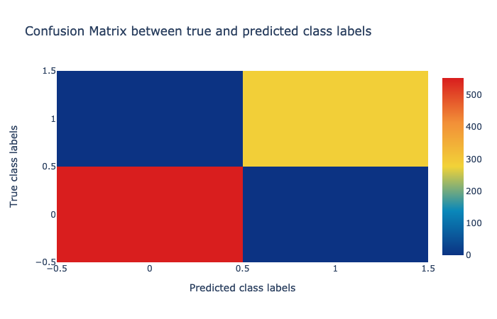
So, we can see that the ensemble methods have a high quality prediction on deciphering whether or not a chemical substance is biodegradable. Surely, the mix of flavors in data brings about all the magic and the classifier is able to perform noticeably better than the isolate models.
References
- Alireza Khanteymoori, Anup Kumar, Simon Bray, 2020 Classification in Machine Learning (Galaxy Training Materials). /training-material/topics/statistics/tutorials/classification_machinelearning/tutorial.html Online; accessed Thu Aug 06 2020
- Batut et al., 2018 Community-Driven Data Analysis Training for Biology Cell Systems 10.1016/j.cels.2018.05.012