Introduction to Deep Learning

2020, Jul 26    

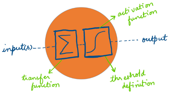
Introduction

Deep Learning convolves state-of-the-art ML theme. Kindly visit this link for my brief presentation from the previous workshop and an example workflow in R .

Assuming a fair understanding for the subject, let's dive right into a data analysis workflow in Galaxy. This exercise is again derived from the official training available here .

Install the repositories- keras_model_config , sklearn_train_test_eval , model_prediction , ml_visualization_ex , and keras_model_builder from the Tool Shed.

Loading Data

The datasets used for this tutorial contain gene expression profiles of humans suffering from two types of cancer - acute myeloid leukemia (AML) and acute lymphoblastic leukemia (ALL). The tutorial aims to differentiate between these two cancer types, predicting a cancer type for each patient, by learning unique patterns in gene expression profiles of patients. The data is divided into 2 parts - one for training and another for prediction. Each part contains two datasets - one has the gene expression profiles and another has labels (the types of cancer). The size of the training data (X_train) is (38, 7129) where 38 is the number of patients and 7129 is the number of genes. The label dataset (y_train) is of size (38, 1) and contains the information of the type of cancer for each patient (label encoding is 0 for ALL and 1 for AML). The test dataset (X_test) is of size (34, 7129) and contains the same genes for 34 different patients. The label dataset for test is y_test and is of size (34, 1). The neural network, which will be formulated in the remaining part of the tutorial, learns on the training data and its labels to create a trained model. The prediction ability of this model is evaluated on the test data (which is unseen during training to get an unbiased estimate of prediction ability).

Let us commence by loading data into a new session. The following could be renamed as X_test, X_train, y_test, and y_train respectively.

1. X_test https://zenodo.org/record/3706539/files/X_test.tsv
2. X_train https://zenodo.org/record/3706539/files/X_train.tsv
3. y_test https://zenodo.org/record/3706539/files/y_test.tsv
4. y_train https://zenodo.org/record/3706539/files/y_train.tsv

Model Structuring

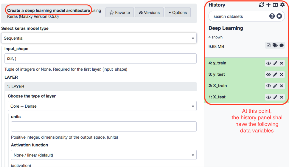
The data in place, we may proceed towards building the model architecture with the following paramaters.

• “Select keras model type”: Sequential
• “input_shape”: (7129, )
- In “LAYER”:
• “1: LAYER”:
• “Choose the type of layer”: Core -- Dense
• “units”: 16
• “Activation function”: elu
• “2: LAYER”:
• “Choose the type of layer”: Core -- Dense
• “units”: 16
• “Activation function”: elu
• “3: LAYER”:
• “Choose the type of layer”: Core -- Dense
• “units”: 1
• “Activation function”: sigmoid

The tool returns a JSON output file with the attributes about the neural networks. The same can be viewed by clicking the "eye" icon. This output goes to the next stage of consolidating the deep learning model with additional parameters as optimiser, loss function, and the number of epochs and batch size (training attributes). The loss function is chosen as binary_crossentropy as the learning task is classification of binary labels (0 and 1).

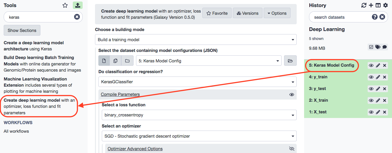
For the next stage, we specify the following constraints.

• “Choose a building mode”: Build a training model
• “Select the dataset containing model configurations (JSON)”: Keras model config (output of Create a deep learning model architecture using Keras tool)
• “Do classification or regression?”: KerasGClassifier
- In “Compile Parameters”:
• “Select a loss function”: binary_crossentropy
• “Select an optimizer”: RMSprop - RMSProp optimizer
- In “Fit Parameters”:
• “epochs”: 10
• “batch_size”: 4

KerasGClassifier is chosen because the learning task is classfication i.e. assigning each patient a type of cancer. The loss function is binary_crossentropy because the labels are discrete and binary (0 and 1).

Training the Deep Learning Model

Install the tool- “Train, Test and Evaluation” and look for the interface as below.

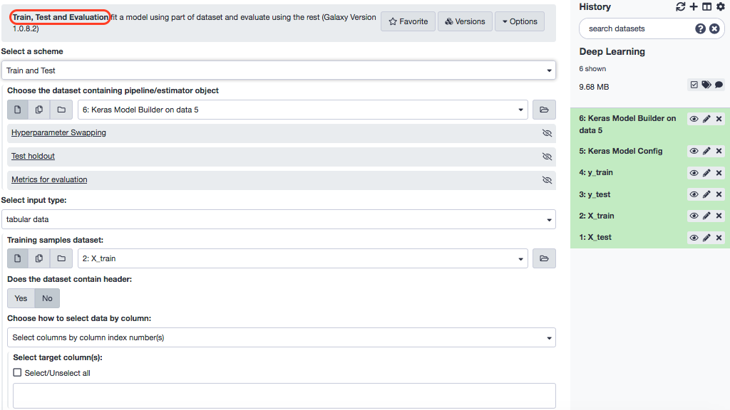
Choose these parameters.

• “Select a scheme”: Train and validate
• “Choose the dataset containing pipeline/estimator object”: Keras model builder (output of Create deep learning model tool)
• “Select input type”: tabular data
• “Training samples dataset”: X_train
• “Does the dataset contain header”: Yes
• “Choose how to select data by column”: All columns
• “Dataset containing class labels or target values”: y_train
• “Does the dataset contain header”: Yes
• “Choose how to select data by column”: All columns

The above execution produces three outputs-

model weights on which the training is premised (Binary HDF5 file)

fitted estimator (ZIP file)

cross-validation accuracy ( tabular file)

In our run, we achieved an accuracy score of 0.8571428656578064 (~ 85%), which is decent.

Testing Prediction Capacity

After training the model, we are tempted to examine if the model is able to make acceptable predictions. We shall execute this model on the test data and study the results. We shall apply the Model Prediction tool, with the following paramaters, for the same.

• “Choose the dataset containing pipeline/estimator object”: Fitted estimator or estimator skeleton (output of Deep learning training and evaluation tool)
• “Choose the dataset containing weights for the estimator above”: Weights trained (output of Create deep learning model tool)
• “Select invocation method”: predict
• “Select input data type for prediction”: tabular data
• “Training samples dataset”: X_test
• “Does the dataset contain header”: Yes
• “Choose how to select data by column”: All columns

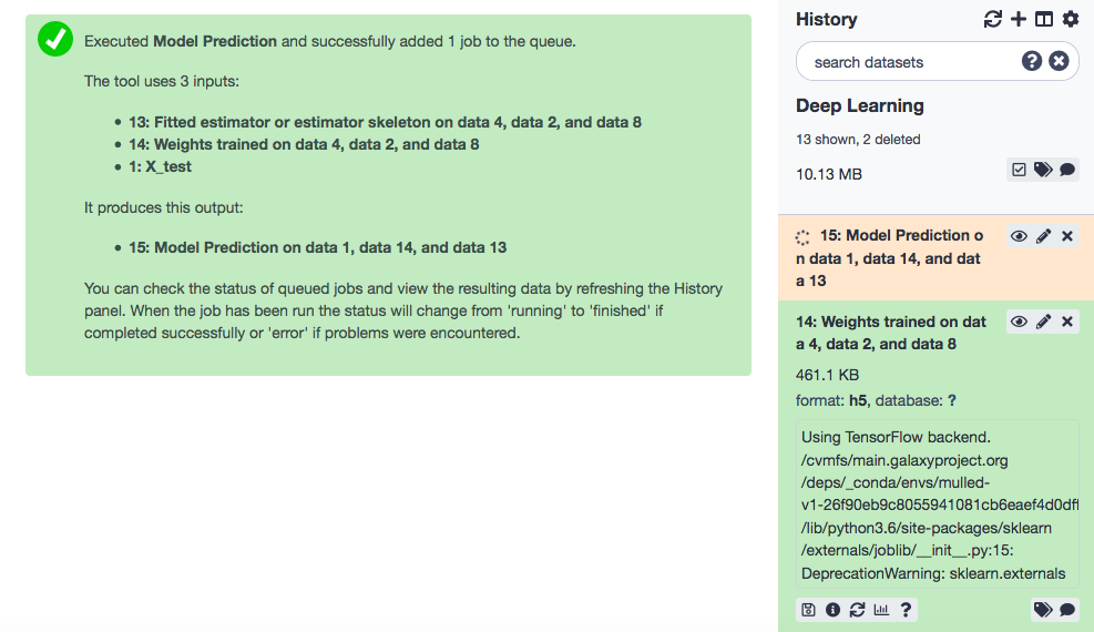
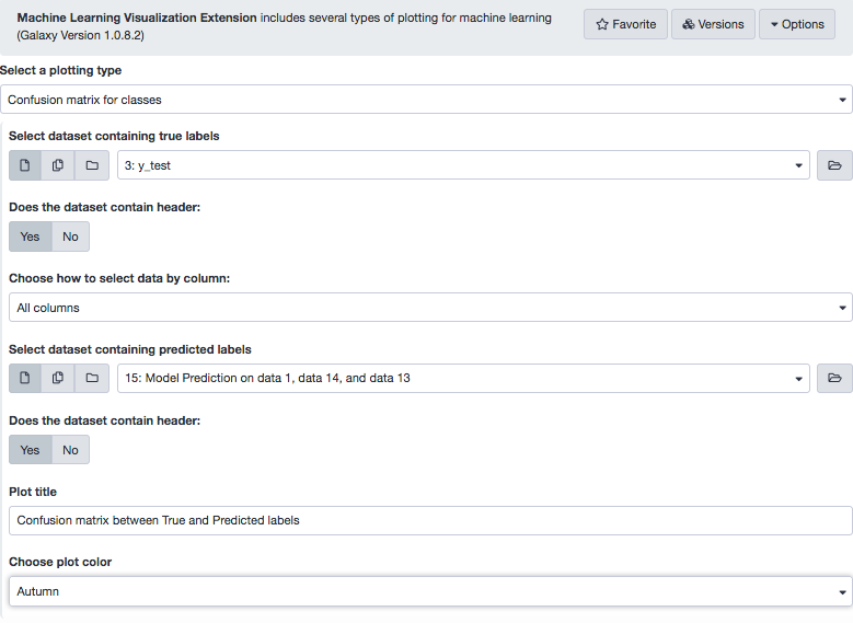
The tool returns predicted labels (in a tabular format) for the test data. Note that 0 represents ALL and 1, AML. It is always good to have a visualization of results to make interpretations more intuitive. A great way to infer the prediction results from a ML model is the confusion matrix , which is a cross-tabulation of the actual and the predicted labels. The tool Machine Learning Visualization Extension helps do that for us.

The following snapshot of the tool interface highlights all the input parameters.

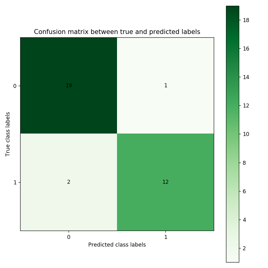
The confusion matrix shows that 19 and 12 cases were correctly predicted for ALL and AML, by the classifier. In the top-right cell, 1 patient who has ALL is predicted having AML. In the bottom-left cell, 2 patients have AML but are predicted suffering from ALL.

References

1. Batut et al., 2018 Community-Driven Data Analysis Training for Biology Cell Systems 10.1016/j.cels.2018.05.012