Regression in Machine Learning

Introduction

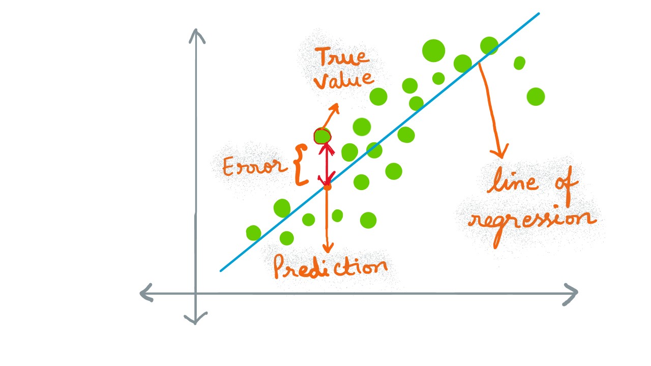
Regression is a technique, extensively used in Machine Learning domain for predicition of continuous values , as an assignment to the target variable, given a series of independent variables. The model learns the input values from an instance (data-row), for each variable/ feature. A line/ curve (regression line) is then attempted to fit the data that is reminiscent of the overall data scatter/ distribution. There are several flavors to regression technique, eg. simple linear regression (fitting straight line to the data, with a dependent/ target variable and an independent variable ), multiple linear regression (series of independent variables and a dependent variable), etc. As can be inferred from the salutation graphic, the better model is the one that is able to accomodate every data point with minimum error, i.e. the true value is as close possible to the predicted value.

Let us recall the attributes of a line from the annals of geometry. A line could be strcutured with a slope and an intercept . These values can be realized as pictured below. Assume a data-point lying in a virtual line; and then there is the regression line. Intuitively, if the equations of both lines are same, then it's a perfect match.

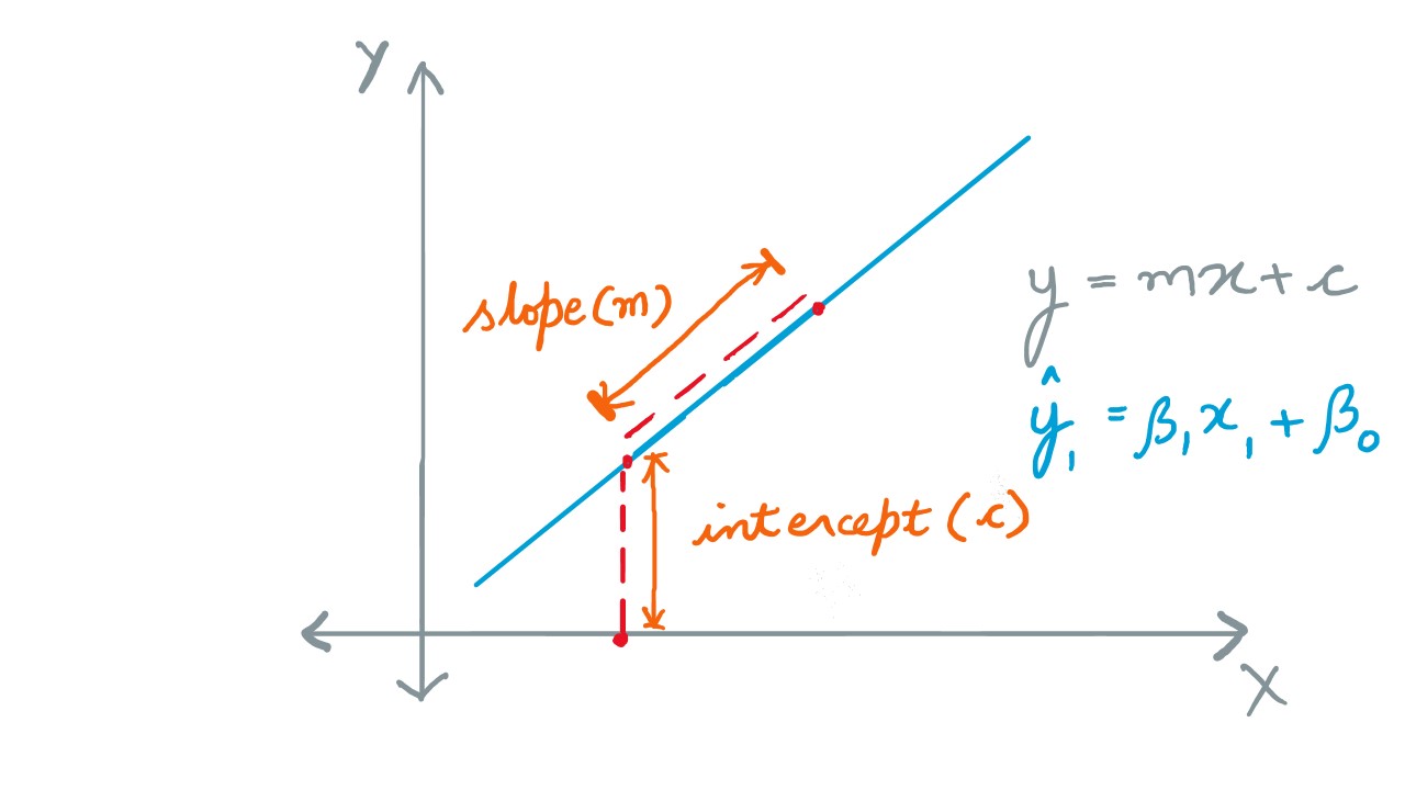
The slope and intercept are the purported coefficients to the equation of a regression line, as for a regular line. If the slope is constant, the only difference between these two lines is that of intercept , meaning thereby that the lines are parallel. In technical terms, this error (difference between actual and predicted value) for all data-points is gauged and optimized using a cost function; cost is the error incurred in prediciting values. The cost function is typically the Mean Squared Error (MSE) or the Sum of Squared Error (SSE) .

It is appropriate to draw a comparison between correlation and regression techniques. While correlation attempts to establish relationships amongst variables, being positively correlated (values following an upward scaling pattern), negatively correlated (values following an downward scaling pattern), or a not correlated at all, regression models the overall data profile by fitting a curve that best defines the pattern.

The case study we use in this exercise is that of age prediction . An exegesis is referred where the DNA methylation profiles were analyzed to predict age of the individuals. This is premised over the dogma that the methylation patterns are dynamic and variable to the age. The CpG sites with the highest correlation to age are selected as the biomarkers (and therefore features for building a regression model).

Let us move to the hands-on now. First, we will fetch the testing and training datasets.

Data

Whole blood samples are collected from humans with their ages falling in the range 18-69 and the best age-correlated CpG sites in the genome are chosen as features. The DNA methylation at the CpG sites offers best biomarking for individuals and their respective age. The training set contains 208 rows corresponding to individual samples and 13 features (age-correlated CpG sites in DNA methylation dataset). The last column is Age. The test set contains 104 rows and the same number of features as the training set. The Age column in the test set is predicted after training on the training set. Another dataset test_rows_labels contains the true age values of the test set which is used to compute scores between true and predicted age. The train_rows contains a column Age which is the label/ target. We will evaluate our model on test_rows and compare the predicted age with the true age in test_rows_labels.

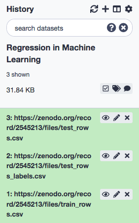
We shall proceed to rename the data to test_rows, test_rows_labels, and train_rows respectively, and confirm that the datatype is tabular.

The age is a real number and also the target variable. It cannot be classified as some discrete value and hence the problem becomes a regression problem rather than a classification task.

Tool Execution

Training the Model

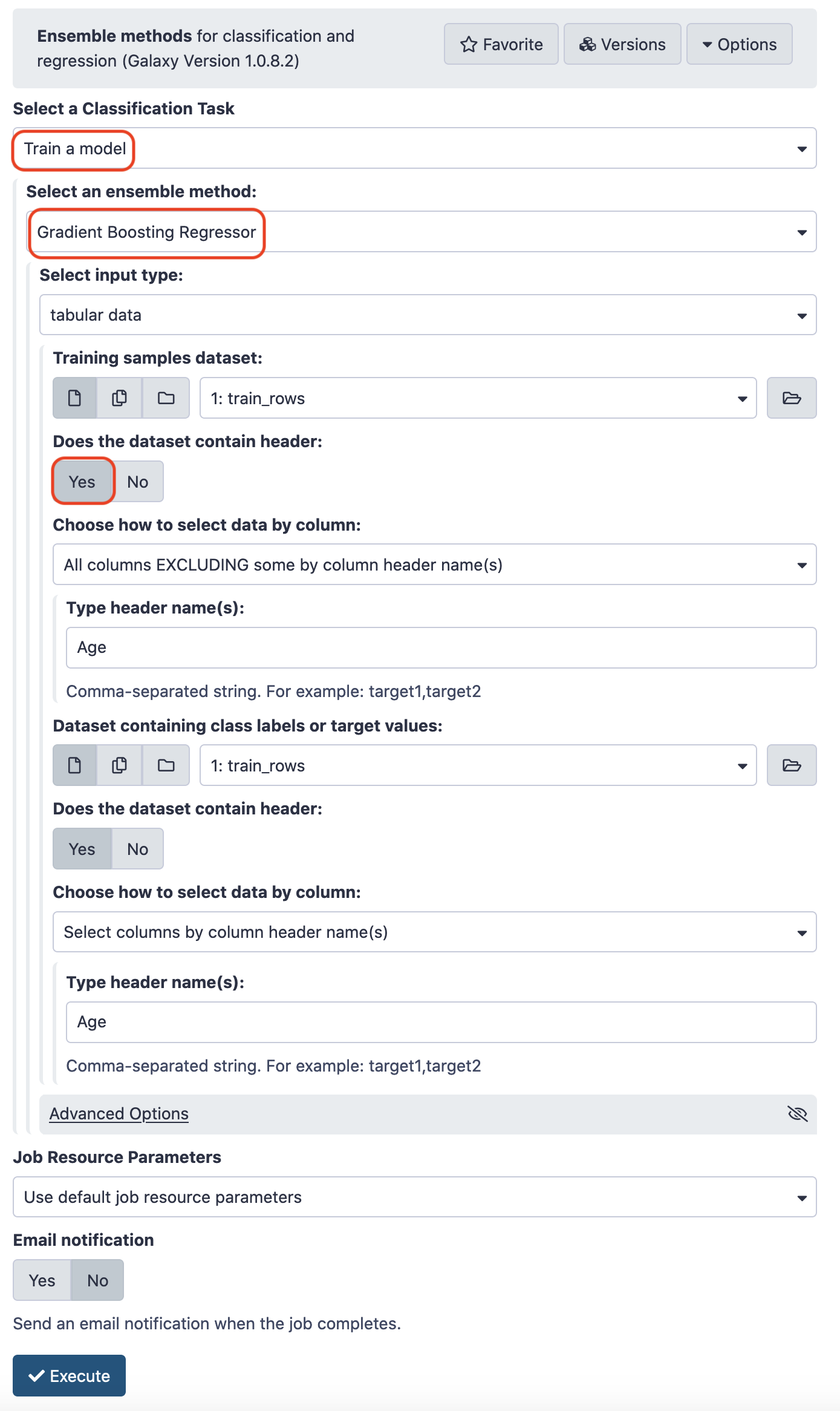
Choose the following paramaters.

“Select a Classification Task” : Train a model
“Select a linear method” : Linear Regression model
“Select input type”: tabular data
param-file “Training samples dataset”: train_rows
param-check “Does the dataset contain header”: Yes
param-select “Choose how to select data by column”: All columns EXCLUDING some by column header name(s)
param-text “Type header name(s)”: Age
param-file “Dataset containing class labels or target values”: train_rows
param-check “Does the dataset contain header”: Yes
param-select “Choose how to select data by column”: Select columns by column header name(s)
param-text “Type header name(s)”: Age

The output is a compressed ZIP file that contains the fitted model. Now that we have the model, we shall try it with the test data and subsequently visualize the results.

Testing the Model

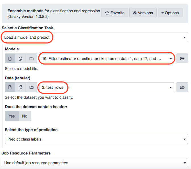
Execute the same tool as above, with the choices as depicted in the screenshot below.

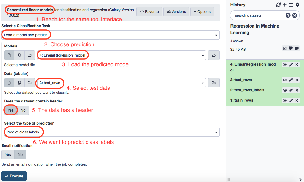
The predicted data is renamed as predicted_data_linear . It contains no header. A dataset called test_rows_labels has the actual labels and contains a header, which we shall remove (use Remove beginning of a file , which is a default tool available in Galaxy, and rename the resulting table to test_rows_labels_without_header ). This is the data we'll be pitting the predicted values against and then compare and visualize the results.

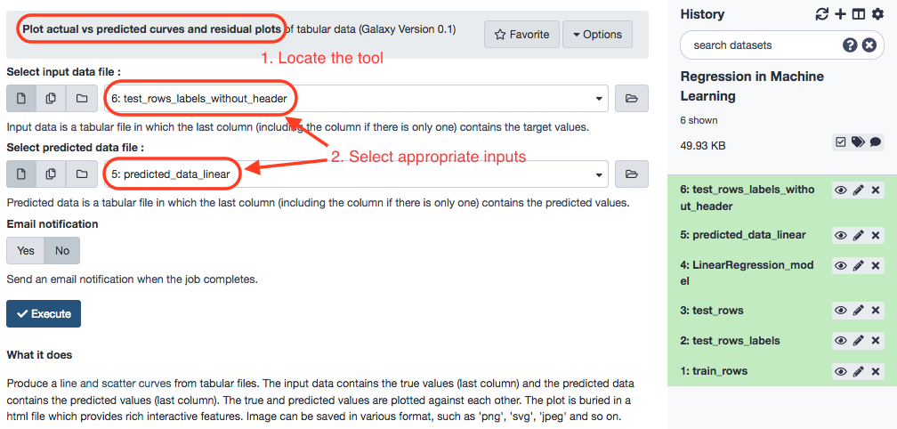
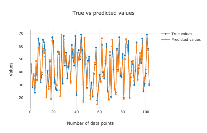
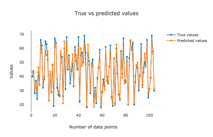
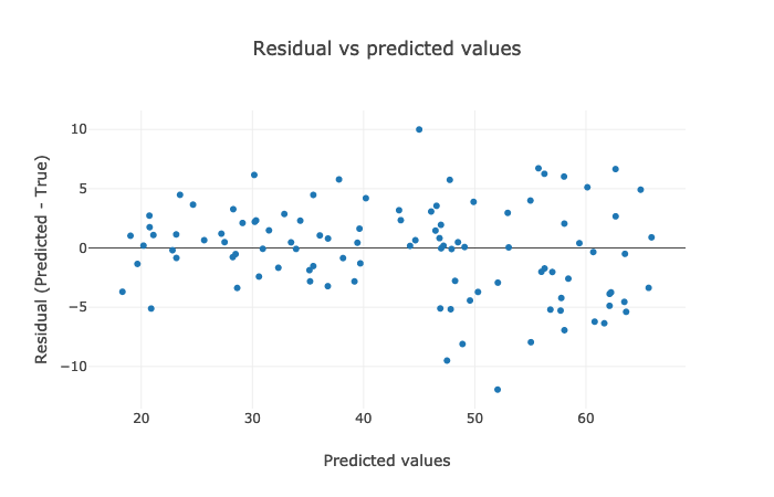
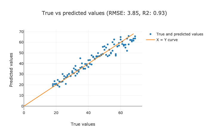
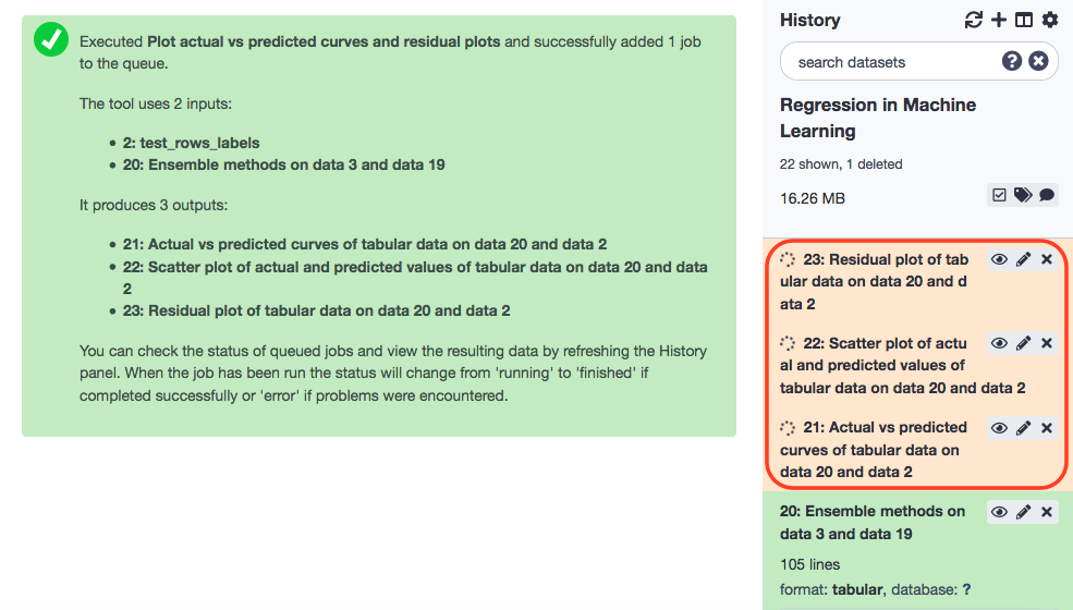
The tool Plot actual vs predicted curves and residual plots is available in the repository plotly_regression_performance_plots . The output from the current run are three plots served as HTML files.

**Figure 1: True vs. Predicted Targets** *The distinctly colored dots represent repsective data-points. Again, lower the difference between actual and preicted values, the better are the results.*

**Figure 2: Residual Plot** *Ideally the scatter should be symmetric across y= 0 and exhibit a random spread.*

**Figure 3: Scatter Plot** *If the prediction is precise, the scatter shall lie close to the line x= y.*

Using Ensemble Methods

Frequently, a single model is a feeble exposition of the data. It is always advisable to work with multiple instances of a model (learner with varying supplements of choice of data-instances, parameters, partitioning, tuning convergence, etc.) and lionize the aggregation of results. A linear regression might not always be the best fit for the data. What if the spread is more concave or convex?

To exemplify, a Random Forest algorithm is a better choice than a Decision Tree . Why? Because multiple trees consistute a forest, and aggregation of many decision trees converges into the output of a random forest. It is an ensemble based classifier and always preferable to employ. Machine Learning is always about the intricacies of statistics (working with sample data to train and test), and so to maximize our chances of a win, it must be ensured that randomness has been cornered as far possible.

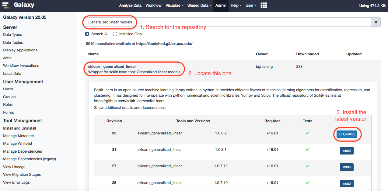
To work with ensemble methods, we shall load the tool Ensemble methods for classification and regression from the repository sklearn_ensemble. We shall be using Gradient Boosting regressor . Make the choices for the paramaters as pictured below.

After training, let's examine the performance of the model on the test data. Prior though, rename the model to gradient_boosting_model. For testing, the parameters could be chosen like below.

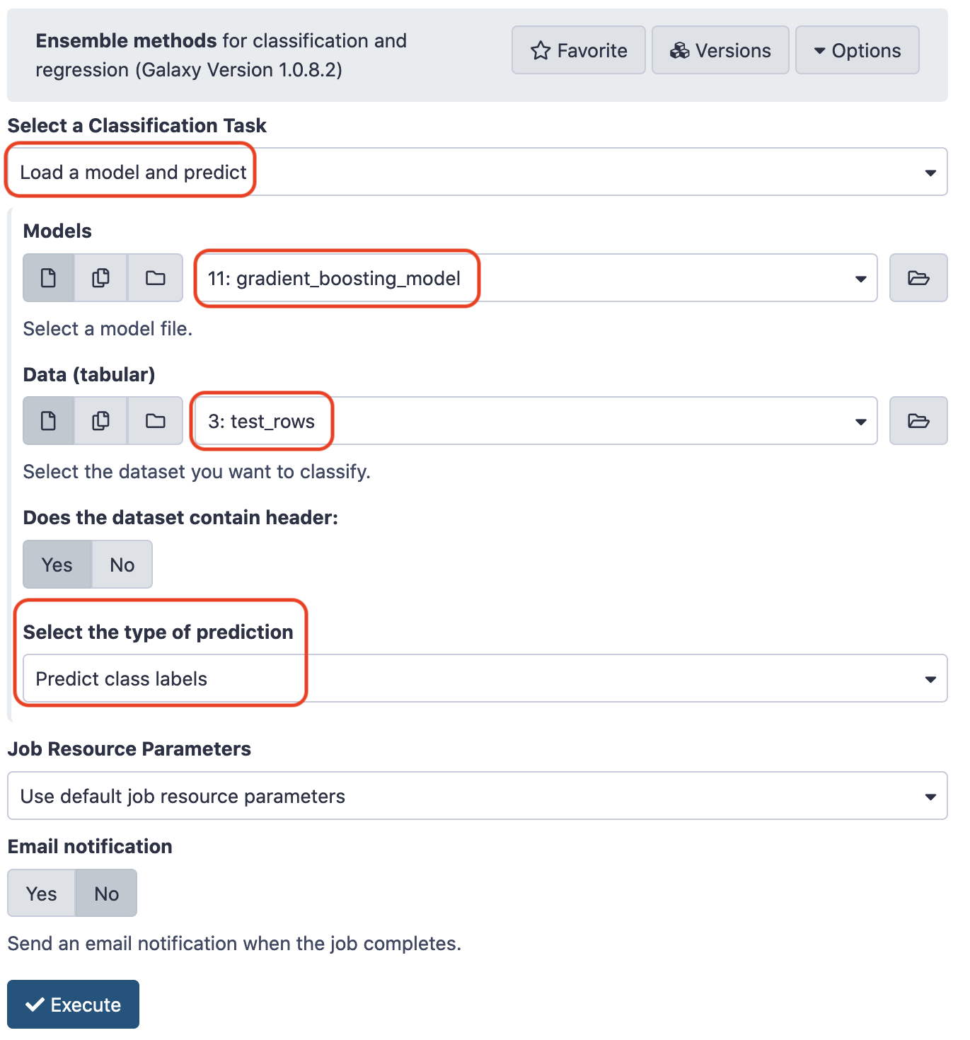
Again, rename the results to predicted_data_gradient_boosting. Now, load the tool Plot actual vs predicted curves and residual plots.

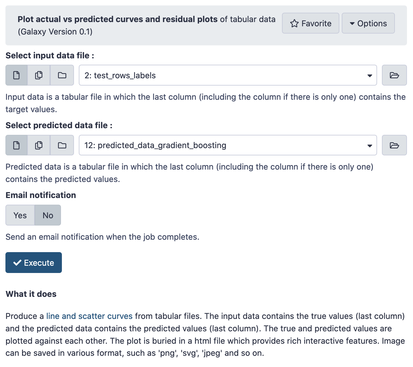
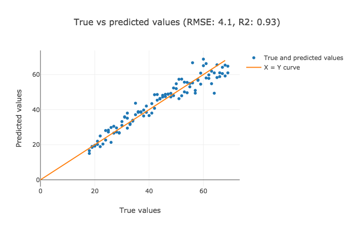
Let's visualize the results. The justification of the results could be reciprocated from the explanations above.

Creating Data Processing Pipeline

To further our analysis, we shall install a tool Pipeline Builder first.

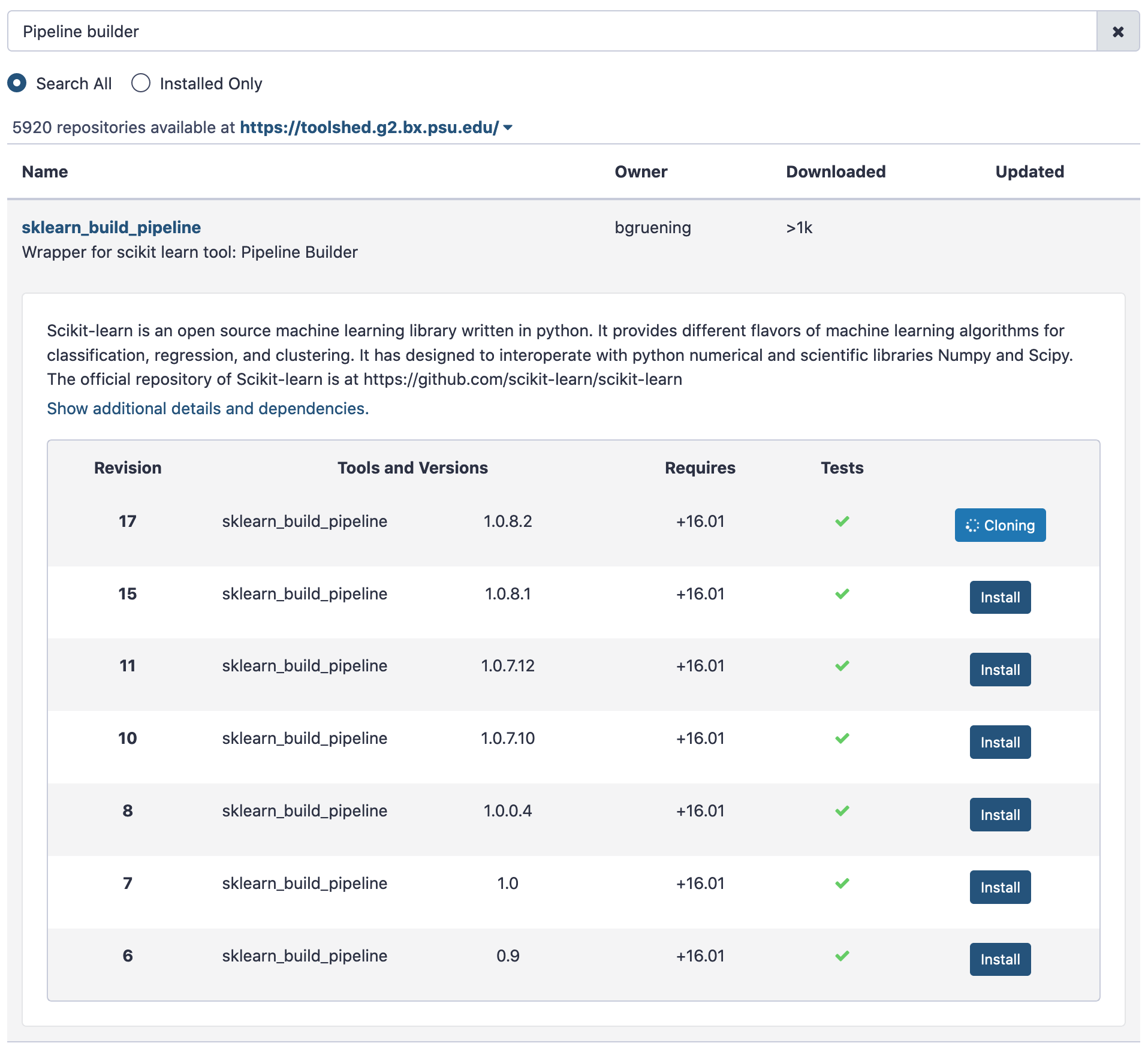
After installation, let us execute the tool with the results we have.

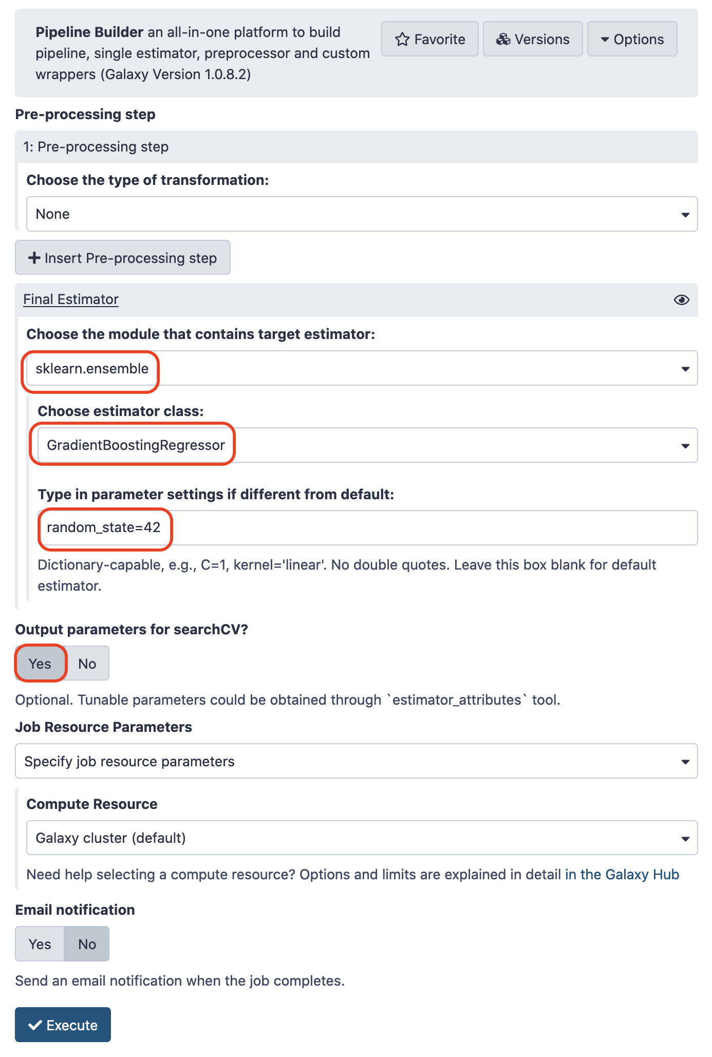
The output is rudimentarily a wrapper that encapsulates this ensemble leaner. The paramaters choosen for this model shall be engendered in a seperate archive. Likewise, we can extend the same pipeline for any other optimum set of arguments. For that we need another tool called Hyperparamater search . We will install it too.

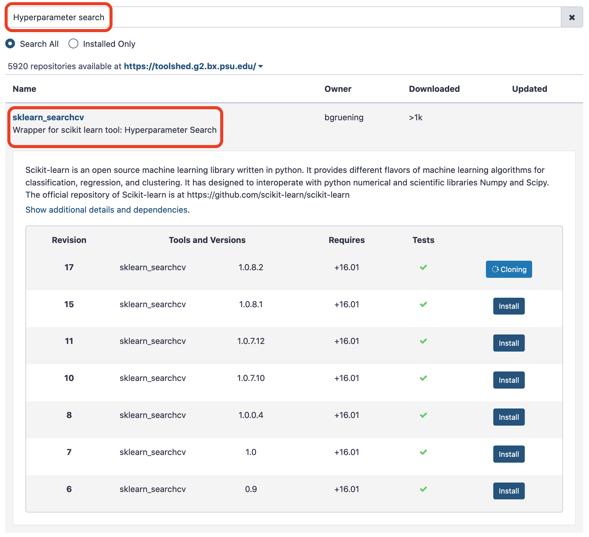
Hyperparameter Search

After creating a pipeline builder, we will use the tool Hyperparameter search to trace the best values for each hyperparameter, so as to establish an optimum model based on the search space chosen for each hyperparameter. We use only one parameter n_estimators of Gradient boosting regressor for this task. This parameter specifies the number of boosting stages the learning process has to go through. The default value of n_estimators for this regressor is 100. However, we are not sure if this gives the best accuracy. Therefore, it is important to try setting this parameter to different values to find the optimal one. We choose some values which are less than 100 and a few more than 100. The hyperparameter search will look for the optimal number of estimators and gives the best-trained model as one of the outputs. This model is used in the next step to predict age in the test dataset.

Install the tool and make the following choices.

“Select a model selection search scheme”: GridSearchCV - Exhaustive search over specified parameter values for an estimator
param-files “Choose the dataset containing pipeline/estimator object”: zipped file (output of Pipeline builder tool)
“Is the estimator a deep learning model?”: No
param-files “Choose the dataset containing parameter names”: tabular file (the other output of Pipeline builder tool)
param-repeat “1: Parameter settings for search”
“Choose a parameter name (with current value)”: n_estimators: 100
“Search list”: [25, 50, 75, 100, 200]
“Select the primary metric (scoring)”: Regression -- 'r2'
“Select the cv splitter”: KFold

There are different ways to split the dataset into training and validation sets. In our tutorial, we will use KFold which splits the dataset into K consecutive parts. It is used for cross-validation. It is set to 5 using another parameter n_splits.

“n_splits”:5
“Whether to shuffle data before splitting”: Yes
“Random seed number” :3111696

It is set to an integer and used to retain the randomness/accuracy when “Whether to shuffle data before splitting” is Yes across successive experiments.

“Raise fit error”:No

While setting different values for a parameter during hyperparameter search, it can happen that wrong values are set, which may generate an error. To avoid stopping the execution of a regressor, it is set to No which means even if a wrong parameter value is encountered, the regressor does not stop running and simply skips that value.

“Select input type”: tabular data
param-files “Training samples dataset”: train_rows tabular file
“Does the dataset contain header”: Yes
“Choose how to select data by column”: All columns EXCLUDING some by column header name(s)
“Type header name(s)”: Age
param-files “Dataset containing class labels or target values”: train_rows tabular file
“Does the dataset contain header”: Yes
“Choose how to select data by column”: Select columns by column header name(s)
“Type header name(s)”: Age
“Whether to hold a portion of samples for test exclusively?”: Nope
“Save best estimator?”: Fitted best estimator or Detailed cv_results_ from nested CV

Exercise

The run will engender two outputs. Analyze the tabular output and ascertain the optimum number of estimators for the gradient boosting regressor.

The other output from the run of Hyperparameter search (zipped file) is the optimized model. Now, to predict the age, we shall execute this model, for probably improvised results.

Next, we shall plot the results again and compare with the existing ones. (Note: The metric R2 is better when closer to 1.0) .

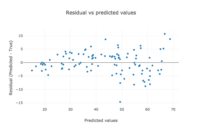
Regression Plots

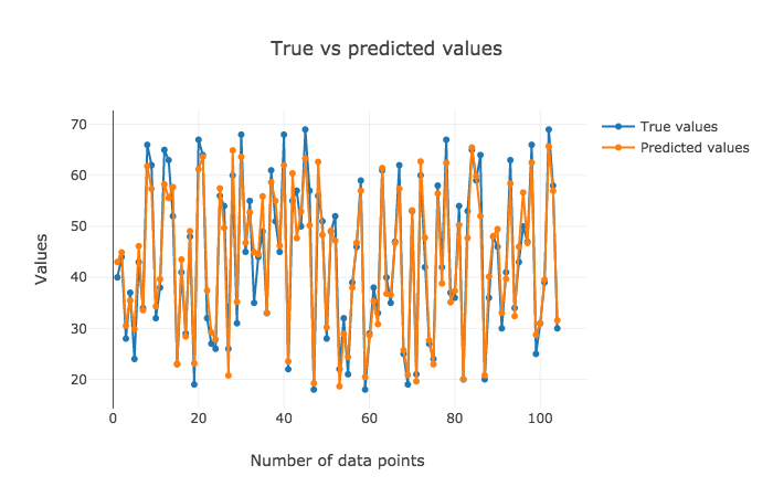
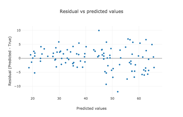
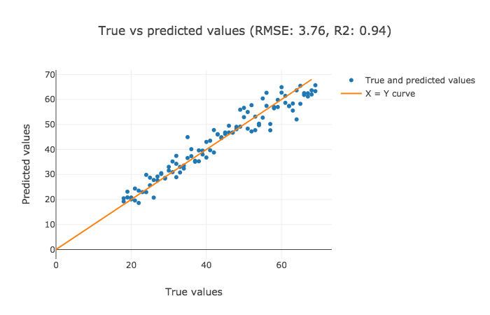
The interpretation for the former two plots has to be made visually, but the latter one highlights RMSE and R2 values that are crispier than before. This is definitely a better version.

References

Alireza Khanteymoori, Anup Kumar, Simon Bray, 2020 Regression in Machine Learning (Galaxy Training Materials). /training-material/topics/statistics/tutorials/regression_machinelearning/tutorial.html Online; accessed Fri Jul 31 2020